Exploring the Tidyverse

Steven Mortimer
January 17, 2017

What is the tidyverse?

These packages can work in harmony because they share common data representations and API design. They strive towards “tidy” data and functions are consistent and easily (human) readable.


It's a lifestyle embodied in a collection of R packages:


More practically the tidyverse

  1. Syncs package versions and warns compatibility
  2. Runs fast - most functions are written in C++
  3. Smarter defaults - No factors in readr::read_csv()!


Tidyverse Core: ggplot2, dplyr, tidyr, tibble, readr, purrr

Other functionality (packages):

  • Importing Data (haven, readxl, httr)
  • Manipulating Data (stringr, lubridate)
  • Modeling Data(modelr, broom)

Reducing Package Confusion


Left Join 2 data.frames

reshape2 package

merge(df1, df2, by.x = 'a1', by.y = 'a2', all.x = TRUE)

data.table package

df2[df1] # must set keys as well

dplyr package

left_join(df1, df2, by=c('a1'='a2'))

Reducing Package Confusion

Warnings when loading plyr after dplyr

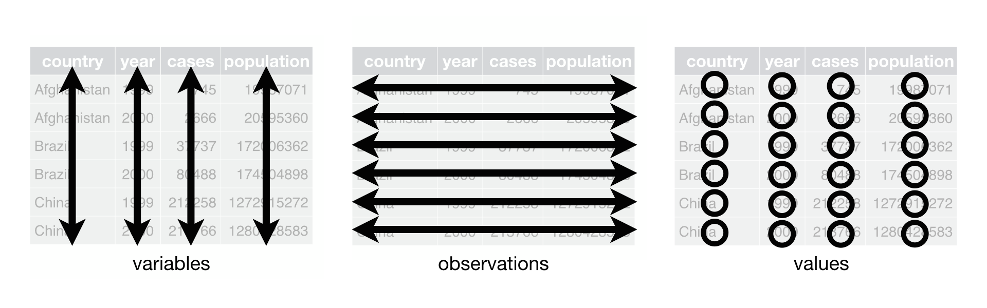
Adhering to "tidy" Principles

Following three rules makes a dataset tidy:

  1. Variables are in columns
  2. Observations are in rows
  3. Values are in cells

Tidying Data

Column headers are values, not variable names and multiple variables are stored in Country

# A tibble: 2 x 4
  Country        `2014` `2015` `2016`
  <chr>           <dbl>  <dbl>  <dbl>
1 Asia-China        100     10     40
2 Europe-Germany    110     15     30
dat %>% 
  gather(-Country, key=Year, value=Data) %>%
  separate(Country, c('Continent', 'Country'))
# A tibble: 6 x 4
  Continent Country Year   Data
  <chr>     <chr>   <chr> <dbl>
1 Asia      China   2014    100
2 Europe    Germany 2014    110
3 Asia      China   2015     10
4 Europe    Germany 2015     15
5 Asia      China   2016     40
6 Europe    Germany 2016     30

What is a tibble?


You've seen it before in dplyr called tbl_df.

tibble is a dedicated package for tbl_df features didn't belong in dplyr package.

What tibbles don't do:

  1. they never create row names
  2. they never change the names of variables
  3. they do not print everything by default
  4. they handle types explicitly (e.g. it never converts strings to factors!)

Consistency! Tibbles return Tibbles

With data frames, [ can return a data.frame or a vector.

is.data.frame(df_dat)
[1] TRUE
df_dat[,2]
[1] 100 110
is.vector(df_dat[,2])
[1] TRUE

With tibbles, [ always returns another tibble.

is.tibble(dat)
[1] TRUE
dat[,2]
# A tibble: 2 x 1
  `2014`
   <dbl>
1    100
2    110
is.tibble(dat[2,2])
[1] TRUE

Pipelines


The pipe, %>%, is a common composition tool that works across all tidyverse packages. It sends the output of the left-hand side (LHS) function to the first argument of the right-hand side (RHS) function.

1:8 %>%
  sum() %>% 
  sqrt()
[1] 6

Why is this important in the tidyverse?

“Consistent and human readable”. Pipelines clearly outline the steps to transform, aggregate, select, etc.

Pipelines - Counts across 2 columns

table(mtcars$cyl, mtcars$am)

     0  1
  4  3  8
  6  4  3
  8 12  2
mtcars %>%
  count(cyl, am) 
# A tibble: 6 x 3
    cyl    am     n
  <dbl> <dbl> <int>
1     4     0     3
2     4     1     8
3     6     0     4
4     6     1     3
5     8     0    12
6     8     1     2

Pipelines - Marginal Proportion

prop.table(table(mtcars$cyl, mtcars$am), margin=1)

            0         1
  4 0.2727273 0.7272727
  6 0.5714286 0.4285714
  8 0.8571429 0.1428571
mtcars %>%
  count(cyl, am) %>%
  group_by(cyl) %>%
  mutate(pct_of_cyl = n / sum(n)) %>%
  ungroup()
# A tibble: 6 x 4
    cyl    am     n pct_of_cyl
  <dbl> <dbl> <int>      <dbl>
1     4     0     3      0.273
2     4     1     8      0.727
3     6     0     4      0.571
4     6     1     3      0.429
5     8     0    12      0.857
6     8     1     2      0.143

Pipelines - Flowing into ggplot

dat %>%
  gather(-Country, key=Year, value=Data) %>%
  separate(Country, c('Continent', 'Country')) %>%
  group_by(Year) %>%
  mutate(Proportion = Data / sum(Data)) %>%
  ggplot(aes(x = Year, y = Proportion, fill = Country)) + 
  geom_bar(stat = "identity") + 
  scale_y_continuous(labels = scales::percent)

Pipelines - API Data Munging

Sample of API Data

movie_list
$movie1
$movie1$genre
[1] "comedy"

$movie1$sales_mm
[1] 28.32


$movie2
$movie2$genre
[1] "romance"

$movie2$sales_mm
[1] 93.14


$movie3
$movie3$genre
[1] "comedy"

$movie3$sales_mm
[1] 41.68

Find Comedy Genre Total Sales

l2 <- lapply(movie_list, data.frame)
final <- do.call(rbind, l2)
sum(subset(final, genre=='comedy')$sales_mm)
[1] 70
final <- plyr::ldply(movie_list, data.frame)
final2 <- plyr::ddply(final, c("genre"), summarise,
                      total_sales = sum(sales_mm))     
subset(final2, genre == 'comedy')
   genre total_sales
1 comedy          70
movie_list %>%
  map_df(., data.frame) %>%
  filter(genre == 'comedy') %>%
  summarize(total_sales = sum(sales_mm))
  total_sales
1          70

Using the "map" function


map is the tidyverse equivalent to many *apply functions in Base R and **ply functions in the plyr package.

map walks through the input, supplying inputs to the function. Various output types can be returned:

  1. map() returns transformed input
  2. map_df() returns a data.frame
  3. map_lgl() map_chr(), map_int() return as certain types

Even Models can be "tidy"

library(broom)
model <- lm(mpg ~ hp, data = mtcars)
tidy(model)
# A tibble: 2 x 5
  term        estimate std.error statistic  p.value
  <chr>          <dbl>     <dbl>     <dbl>    <dbl>
1 (Intercept)  30.1       1.63       18.4  6.64e-18
2 hp           -0.0682    0.0101     -6.74 1.79e- 7
summary(model)$r.squared # Base R way
[1] 0.6024373
library(modelr)
rsquare(model, mtcars) # tidyverse way
[1] 0.6024373

Bootstrapped 95% CI

We know hp has a statistically signficant relationship to mpg

β = -0.06823, t(30) = -6.742, p < .001

What if we could not compute the standard error or CI? Alternatively, the test for significance could be bootstrapped.

bootstrap(mtcars, 100) %>%
  mutate(model = map(strap, ~ lm(mpg ~ hp, data = .))) %>% 
  mutate(tidy_model = map(model, tidy)) %>% 
    mutate(hp_estimate = map_dbl(tidy_model, . %>% 
                                   filter(term == 'hp') %>% 
                                   .$estimate)) %>%
    summarize(lower = quantile(hp_estimate, .025),
              upper = quantile(hp_estimate, .975))
# A tibble: 1 x 2
    lower   upper
    <dbl>   <dbl>
1 -0.0973 -0.0460

Fitting Partitioned Models


Fit a separate linear regression by cyl:

mtcars %>% 
  split(.$cyl) %>%
  map(~ lm(mpg ~ hp, data = .)) %>%
  map_df(tidy, .id = "cylinder") %>%
  arrange(term)
# A tibble: 6 x 6
  cylinder term         estimate std.error statistic   p.value
  <chr>    <chr>           <dbl>     <dbl>     <dbl>     <dbl>
1 4        (Intercept)  36.0        5.20       6.92  0.0000693
2 6        (Intercept)  20.7        3.30       6.26  0.00153  
3 8        (Intercept)  18.1        2.99       6.05  0.0000574
4 4        hp           -0.113      0.0612    -1.84  0.0984   
5 6        hp           -0.00761    0.0266    -0.286 0.786    
6 8        hp           -0.0142     0.0139    -1.02  0.326    

Resources

Welcome to the tidyverse lifestyle!